


M1 BBS ACP
From silico.biotoul.fr
Contents |
Analyse en composantes principales
Objectif : Réduire le nombre de dimensions de l'espace d'observation = obtenir une projection en perdant un minimum d'informations.
Applications :
- grand nombre de variables que l'on cherche à visualiser en 2 à 3 dimensions
- dessin de graphes
ici schéma changement de repère (2 dimensions)
 Principe : trouver les axes sur lesquels on a un maximum de dispersion = plus de représentativité / moins de perte d'informations
Choix de l'origine
Prendre le centre de gravité du nuage.
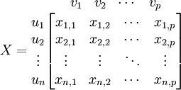
Données :
-
 individus
  points dans l'espace à p dimensions.
-
 variables
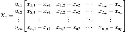
Centre de gravité : 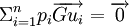 avec pi le poids de chaque dimension
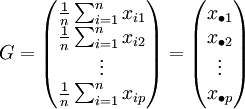
On prendra G comme nouvelle origine.
données centrées
Mesure de dispersion = Inertie
Inertie par rapport à un point (le centre de gravité)

avec 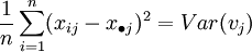
on a 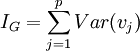
L'inertie par rapport au centre de gravité revient à la somme des variances de chaque variable
Inertie par rapport à un axe
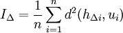
mesure la proximité du nuage des individus à l'axe.
ici figure
Inertie par rapport à un sous-espace vectoriel
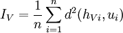 C'est pareil.