


M1 BBS ACP
From silico.biotoul.fr
m (Created page with '= Analyse en composantes principales = '''Objectif :''' Réduire le nombre de dimensions de l'espace d'observation = obtenir une projection en perdant un minimum d'informations.…') |
m (→Recherche de \Delta_1 passant par G d'inertie minimum) |
||
| (4 intermediate revisions not shown) | |||
| Line 6: | Line 6: | ||
* grand nombre de variables que l'on cherche à visualiser en 2 à 3 dimensions | * grand nombre de variables que l'on cherche à visualiser en 2 à 3 dimensions | ||
* dessin de graphes | * dessin de graphes | ||
| - | |||
| - | |||
| - | |||
| - | |||
| - | |||
<math>\Rightarrow</math> '''Principe :''' trouver les axes sur lesquels on a un maximum de dispersion = plus de représentativité / moins de perte d'informations | <math>\Rightarrow</math> '''Principe :''' trouver les axes sur lesquels on a un maximum de dispersion = plus de représentativité / moins de perte d'informations | ||
| Line 38: | Line 33: | ||
| - | Centre de gravité : | + | Centre de gravité : <math>\Sigma^n_{i=1} p_i \overrightarrow{Gu_i} = \overrightarrow{0}</math> avec ''p<sub>i</sub>'' le poids de chaque dimension |
| + | |||
<math> | <math> | ||
G = \begin{pmatrix} | G = \begin{pmatrix} | ||
| - | \frac{1}{n} \ | + | \frac{1}{n} \sum_{i=1}^n x_{i1} \\ |
| - | \frac{1}{n} \ | + | \frac{1}{n} \sum_{i=1}^n x_{i2} \\ |
\vdots \\ | \vdots \\ | ||
| - | \frac{1}{n} \ | + | \frac{1}{n} \sum_{i=1}^n x_{ip} |
\end{pmatrix} | \end{pmatrix} | ||
= \begin{pmatrix} | = \begin{pmatrix} | ||
| Line 74: | Line 70: | ||
\end{bmatrix} | \end{bmatrix} | ||
</math> | </math> | ||
| + | |||
| + | == Mesure de dispersion : Inertie == | ||
| + | === Inertie par rapport à un point (le centre de gravité) === | ||
| + | |||
| + | <math>I_G = \frac{1}{n} \sum_{i=1}^n d^2(G, u_i) = \frac{1}{n}\sum_{i=1}^n \sum_{j=1}^p (x_{ij} - x_{\bullet j})^2 | ||
| + | = \sum_{j=1}^p \frac{1}{n}\sum_{i=1}^n (x_{ij} - x_{\bullet j})^2 | ||
| + | </math> | ||
| + | |||
| + | avec <math>\frac{1}{n}\sum_{i=1}^n (x_{ij} - x_{\bullet j})^2 = Var(v_j)</math> | ||
| + | |||
| + | on a <math>I_G = \sum_{j=1}^p Var(v_j)</math> | ||
| + | |||
| + | <math>\Rightarrow</math> L'inertie par rapport au centre de gravité revient à la somme des variances de chaque variable | ||
| + | |||
| + | === Inertie par rapport à un axe === | ||
| + | |||
| + | <math>I_\Delta = \frac{1}{n}\sum_{i=1}^n d^2(h_{\Delta i}, u_i) | ||
| + | </math> | ||
| + | |||
| + | <math>\rightarrow</math> mesure la proximité du nuage des individus à l'axe. | ||
| + | |||
| + | [[Image:projection.orthogonale.png]] | ||
| + | |||
| + | === Inertie par rapport à un sous-espace vectoriel === | ||
| + | |||
| + | <math>I_V = \frac{1}{n} \sum_{i=1}^n d^2(h_{Vi}, u_i)</math> C'est pareil. | ||
| + | |||
| + | === Décomposition de l'inertie totale === | ||
| + | |||
| + | <math>V^*</math> le complémentaire orthogonal de <math>V</math> | ||
| + | |||
| + | [[Image:inertie.portee.par.l.axe.png]] | ||
| + | |||
| + | on a <math>I_G = I_{V} + I_{V^*}</math> | ||
| + | |||
| + | En projetant sur <math>V</math>, on perd l'inertie mesurée par <math>I_{V}</math> et il ne reste plus que celle mesurée par <math>I_{V^*}</math> | ||
| + | |||
| + | |||
| + | |||
| + | == Recherche de <math>\Delta_1</math> passant par ''G'' d'inertie minimum == | ||
| + | |||
| + | maximise <math>\Delta_1^*</math> avec <math>\overrightarrow{Ga_1}</math> vecteur unitaire de <math>\Delta_1^*</math> | ||
| + | |||
| + | |||
| + | |||
| + | <math>d^2(G, h_{\Delta_1^*i}) = \langle \overrightarrow{Gu_i}, \overrightarrow{Ga_1} \rangle ^2 | ||
| + | = a_1^T U_{ci} U_{ci}^T a_1 | ||
| + | </math> | ||
| + | |||
| + | |||
| + | |||
| + | donc <math>I_{\Delta_1^*} = \frac{1}{n} \sum_{i=1}^n a_1^T U_{ci} U_{ci}^T a_1 | ||
| + | = a_1^T \frac{1}{n} \sum_{i=1}^n U_{ci} U_{ci}^T a_1 | ||
| + | </math> | ||
| + | |||
| + | |||
| + | |||
| + | on reconnaît la matrice de variance-covariance <math>\Sigma = \frac{1}{n} \sum_{i=1}^n U_{ci} U_{ci}^T</math> | ||
| + | |||
| + | |||
| + | |||
| + | donc <math>I_{\Delta_1^*} = a_1^T \Sigma a_1</math> | ||
| + | |||
| + | |||
| + | et <math>\parallel \overrightarrow{G_{a_1}} \parallel = a_1^T a_1 = 1</math> (vecteur unitaire) | ||
| + | |||
| + | |||
| + | D'où la recherche du maximum : trouver <math>a_1</math> tel que <math>a_1^T \Sigma a_1</math> soit maximum (recherche l'optimum d'une fonction à plusieurs variables) | ||
| + | |||
| + | <math>g(a_1) = g( a_{11}, a_{12}, ..., a_{1p}) = a_1^T \Sigma a_1 - \lambda_ç1(a_1^Ta_1 -1) </math> | ||
| + | |||
| + | |||
| + | <math>\rightarrow</math> d'après la méthode des multiplicateurs de Lagrange | ||
| + | |||
| + | <math>\rightarrow</math> dérivées partielles de <math>g(a_1)</math>, en utilisant la dérivée matricielle | ||
| + | |||
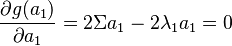
| + | <math>\frac{\partial g(a_1)}{\partial a_1} = 2 \Sigma a_1 - 2 \lambda_1a_1 = 0</math> | ||
| + | |||
| + | |||
| + | donc | ||
| + | |||
| + | <math> | ||
| + | \begin{cases} | ||
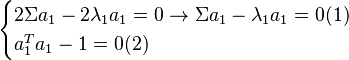
| + | 2 \Sigma a_1 - 2 \lambda_1a_1 = 0 \rightarrow \Sigma a_1 - \lambda_1 a_1 = 0 (1)\\ | ||
| + | a_1^T a_1 - 1 = 0 (2)\\ | ||
| + | \end{cases} | ||
| + | </math> | ||
| + | |||
| + | |||
| + | <math>(1) \leftrightarrow A x = \lambda x</math> ou <math>\Sigma a_1 = \lambda_1 a_1</math> d'où <math>a_1</math> vecteur propre de <math>\Sigma</math> associé à la valeur propre <math>\lambda_1</math> | ||
| + | |||
| + | |||
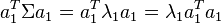
| + | En multipliant à gauche par <math>a_1^T</math> on a | ||
| + | |||
| + | <math>a_1^T \Sigma a_1 = a_1^T \lambda_1 a_1 = \lambda_1 a_1^T a_1</math> avec <math>(2)</math> on <math> = I_{\Delta_1^*}</math> que l'on cherche à maximiser. | ||
| + | |||
| + | |||
| + | Donc <math>\lambda_1</math> est la plus grande valeur propre de la matrice <math>\Sigma</math> et <math>\lambda_1 = I_{\Delta_1^*}</math> | ||
Current revision as of 09:34, 8 October 2018
Contents |
Analyse en composantes principales
Objectif : Réduire le nombre de dimensions de l'espace d'observation = obtenir une projection en perdant un minimum d'informations.
Applications :
- grand nombre de variables que l'on cherche à visualiser en 2 à 3 dimensions
- dessin de graphes
 Principe : trouver les axes sur lesquels on a un maximum de dispersion = plus de représentativité / moins de perte d'informations
Choix de l'origine
Prendre le centre de gravité du nuage.
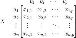
Données :
-
 individus
  points dans l'espace à p dimensions.
-
 variables
Centre de gravité : 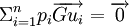 avec pi le poids de chaque dimension
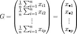
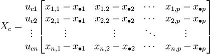
On prendra G comme nouvelle origine.
données centrées
Mesure de dispersion : Inertie
Inertie par rapport à un point (le centre de gravité)

avec 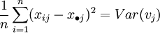
on a 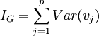
L'inertie par rapport au centre de gravité revient à la somme des variances de chaque variable
Inertie par rapport à un axe
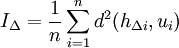
mesure la proximité du nuage des individus à l'axe.

Inertie par rapport à un sous-espace vectoriel
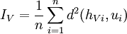 C'est pareil.
Décomposition de l'inertie totale
V * le complémentaire orthogonal de V

on a 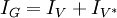
En projetant sur V, on perd l'inertie mesurée par IV et il ne reste plus que celle mesurée par 
Recherche de Δ1 passant par G d'inertie minimum
maximise  avec
avec  vecteur unitaire de

donc 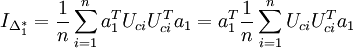
on reconnaît la matrice de variance-covariance 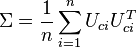
donc 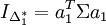
et 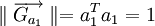 (vecteur unitaire)
D'où la recherche du maximum : trouver a1 tel que  soit maximum (recherche l'optimum d'une fonction à plusieurs variables)

d'après la méthode des multiplicateurs de Lagrange
dérivées partielles de g(a1), en utilisant la dérivée matricielle
donc
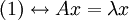 ou Σa1 = λ1a1 d'où a1 vecteur propre de Σ associé à la valeur propre λ1
En multipliant à gauche par  on a
on a
 avec (2) on
  que l'on cherche à maximiser.
Donc λ1 est la plus grande valeur propre de la matrice Σ et 